toWebSite/ directory, unless stated otherwise. Setup and complete workflow · Original Markdown.Coupled-pendulum examples at fixed coupling
All examples use epsilon = 0.1 and the default physical parameters in coupled_pendula.py: m1 = m2 = 1, l1 = 1, l2 = 1.3, a = 3, g = k = 1. State ordering is (q1, q2, p1, p2); angles are in radians and the last two coordinates are canonical momenta, not angular velocities. The coupling is fixed, but the examples have different energies.
| Behaviour | Initial state | Energy H | Suggested display time |
|---|---|---|---|
| Chaotic | (0, 0, 2, 1) |
2.295857988166 | 1000 |
| Libration | (0.8, -0.4, 0, 0) |
0.474283475334 | 400 |
| Periodic | (0.3, -0.0888544167980643, 0, 0) |
0.057939567392 | 120 |
| Quasiperiodic rotations | (0, 0, 3, -4) |
9.233727810651 | 400 |
Libration means bounded angular oscillation. It overlaps with the other classifications: the libration example is numerically quasiperiodic, and the periodic example also librates. The rotational quasiperiodic example has the pendulums turning in opposite directions.
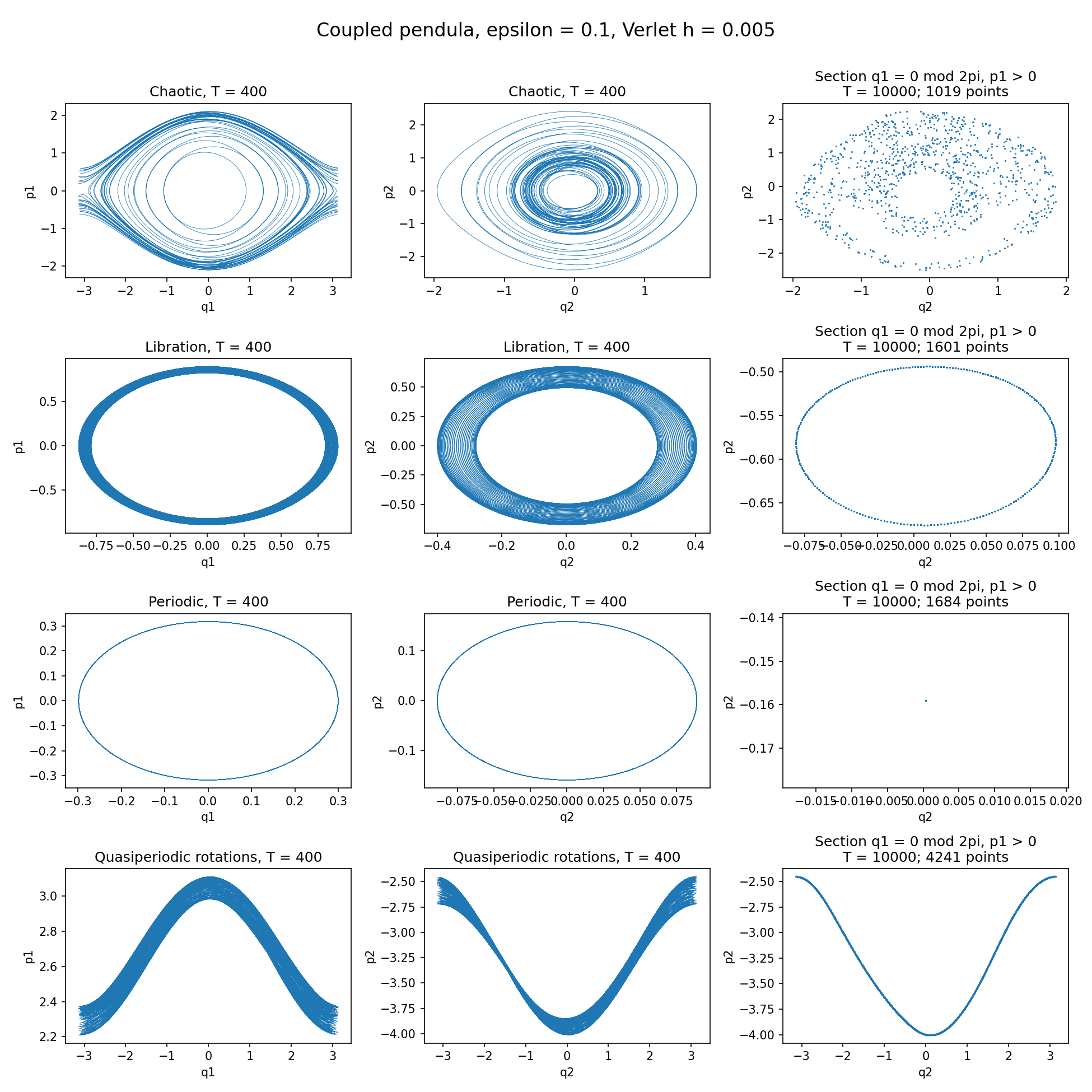
The left and middle columns show phase projections to T = 400; the right column shows Poincare sections to T = 10000. All panels use h = 0.005.
Run the examples
Run a command from the project directory, then click Run in the window. The --initial-state option selects the exact coordinates, avoiding mouse placement errors, which matter especially for the periodic orbit.
# Chaotic
python3 codes/coupled_pendula.py --epsilon 0.1 --duration 1000 --initial-state 0 0 2 1

# Libration
python3 codes/coupled_pendula.py --epsilon 0.1 --duration 400 --initial-state 0.8 -0.4 0 0

# Periodic
python3 codes/coupled_pendula.py --epsilon 0.1 --duration 120 --initial-state 0.3 -0.0888544167980643 0 0

# Quasiperiodic rotations
python3 codes/coupled_pendula.py --epsilon 0.1 --duration 400 --initial-state 0 0 3 -4
These commands use the default Verlet step --dt 0.01. Add --dt 0.005 for smaller discretization error. Full phase projections can look thick for both quasiperiodic and chaotic trajectories; they are not Poincare sections.
Classification and numerical checks
The selected trajectories were integrated with the project’s integrateTrajectory function to T = 10000, with both h = 0.01 and h = 0.005. Poincare sections used q1 = 0 modulo 2*pi, p1 > 0, with linear interpolation between integration steps.
Chaotic
For (0, 0, 2, 1), the Poincare section is a scattered two-dimensional cloud. Pendulum 1 exhibits irregular librations and rotations. Pendulum 2 remains confined, consistent with the energy being below its gravitational barrier 2.6.
Finite-time largest Lyapunov estimates, obtained by evolving a nearby orbit and renormalizing its separation to 1e-7 every time unit, were:
| T | h = 0.01 | h = 0.005 |
|---|---|---|
| 1000 | 0.08160 | 0.08376 |
| 2000 | 0.09483 | 0.08333 |
| 5000 | 0.10154 | 0.08090 |
| 10000 | 0.08054 | 0.07546 |
The initial perturbation direction was (0.37, -0.51, 0.63, 0.45), normalized in the Euclidean norm of the canonical coordinates. Persistence of a positive estimate under longer integration and step refinement supports chaos; the precise finite-time value varies as the orbit explores the chaotic region.
Libration
For (0.8, -0.4, 0, 0), confinement follows directly from energy conservation: the kinetic and spring energies are nonnegative, and reaching q1 = +/-pi requires H >= 2, while reaching q2 = +/-pi requires H >= 2.6. Here H = 0.474283475334, so neither pendulum can leave its initial well.
At h = 0.005, sampled angle ranges over T = 10000 were approximately q1 in [-0.87130, 0.88735] and q2 in [-0.40000, 0.40425]. The Poincare points lie on a closed curve, and the finite-time Lyapunov estimate decreases from 0.00427 at T = 1000 to 0.000652 at T = 10000, consistent with quasiperiodic libration.
Periodic
For (0.3, -0.0888544167980643, 0, 0), the period of the continuous system is
P = 5.938156672603949This is a nontrivial nonlinear periodic orbit. It was obtained by fixing q1(0) = 0.3, setting both initial momenta to zero, and solving for q2(0) and a half-period tau such that both momenta vanish again at tau. Time reversibility then closes the orbit at P = 2*tau. The shooting seed was the higher-frequency linear normal mode at the origin.
Using SciPy DOP853 for the exact vector field, with rtol = 3e-14 and atol = 3e-15, the full-period infinity-norm closure residual was 3.8e-14 or less. Verlet closure errors over the same period were approximately 9.19e-6 and 2.30e-6, with constant steps just below 0.01 and 0.005 respectively, chosen to land exactly at P. Thus the supplied coordinates describe the continuous periodic orbit to numerical accuracy; the fixed-step GUI trajectory has the expected discretization error.
Quasiperiodic rotations
For (0, 0, 3, -4), the Poincare section follows a smooth invariant-looking curve, with both pendulums rotating in opposite directions. Weighted time averages of qdot = p/inertia, at h = 0.005, give angular rotation rates
omega1 =  2.66491636
omega2 = -1.88464031
omega1 / omega2 = -1.4140185489
These averages use the smooth weight exp(-1/(s*(1-s))), with normalized time 0 < s < 1. The frequency ratio agrees between the first and second 5000-time-unit halves to about 2.5e-10. At h = 0.01 it is -1.4140181676, showing a small discretization shift. The finite-time Lyapunov estimate at h = 0.005 decreases from 0.00678 at T = 1000 to 0.00134 at T = 10000. Together these diagnostics support quasiperiodicity; finite-time computations do not prove an irrational frequency ratio or the existence of an invariant torus.
Energy-error check
Maximum abs(H(t)-H(0))/(1+abs(H(0))) over the full integrations:
| Example | h = 0.01 | h = 0.005 |
|---|---|---|
| Chaotic | 1.52e-5 | 3.80e-6 |
| Libration | 8.50e-6 | 2.12e-6 |
| Periodic | 1.54e-6 | 3.84e-7 |
| Quasiperiodic rotations | 2.25e-5 | 5.61e-6 |
The approximately fourfold reduction is consistent with the second-order Störmer–Verlet scheme.